Microsoft Excel is the spreadsheet program in Microsoft Office.
Microsoft Excel is a spreadsheet developed by Microsoft for Windows, macOS, Android and iOS. It features calculation or computation capabilities, graphing tools, pivot tables, and a macro programming language called Visual Basic for Applications. Excel forms part of the Microsoft Office suite of software
Microsoft Excel enables users to format, organize and calculate data in a spreadsheet. By organizing data using software like Excel, data analysts and other users can make information easier to view as data is added or changed. Excel contains a large number of boxes called cells that are ordered in rows and columns.
A spreadsheet is a type of application program which manipulates numerical and string data in rows and columns of cells. The value in a cell can be calculated from a formula which can involve other cells.
A value is recalculated automatically whenever a value on which it depends changes. Different cells may be displayed with different formats.
Microsoft Excel has the basic features of all spreadsheets, using a grid of cells arranged in numbered rows and letter-named columns to organize data manipulations like arithmetic operations. It has a battery of supplied functions to answer statistical, engineering, and financial needs
Workbook
- A booklet containing problems and exercises that a student may work directly on the pages.
- A manual containing operating instructions, as for an appliance or machine.
- A book in which a record is kept of work proposed or accomplished.
Worksheet
A sheet of paper with multiple columns; used by an accountant to assemble figures for financial statements. A piece of paper recording work planned or done on a project.
You start Excel from the Start menu in Windows. Click the Start button, click All Programs, click Microsoft Office, and then click Microsoft Excel 2010.
The Excel program window has the same basic parts as all Office programs: the title bar, the Quick Access Toolbar, the Ribbon, Backstage view, and the status bar.
Parts of the Worksheet
Exploring Worksheet
Each workbook contains three worksheets by default. The worksheet displayed in the work area is the active worksheet.
- Columns appear vertically and are identified by letters. Rows appear horizontally and are identified by numbers.
- A cell is the intersection of a row and a column. Each cell is identified by a unique cell reference.
- The cell in the worksheet in which you can type data is called the active cell.
- The Name Box, or cell reference area, displays the cell reference of the active cell.
- The Formula Bar displays a formula when a worksheet cell contains a calculated value.
- A formula is an equation that calculates a new value from values currently in a worksheet.
Opening an Existing Workbook
Opening a workbook means loading an existing workbook file from a drive into the program window.
To open an existing workbook, you click the File tab on the Ribbon to display Backstage view, and then click Open in the navigation bar. The Open dialog box appears.
Saving a Workbook
- The Save command saves an existing workbook, using its current name and save location.
- The Save As command lets you save a workbook with a new name or to a new location.
Moving the Active Cell in a Worksheet
- The easiest way to change the active cell in a worksheet is to move the pointer to the cell you want to make active and click.
- You can display different parts of the worksheet by using the mouse to drag the scroll box in the scroll bar to another position.
- You can also move the active cell to different parts of the worksheet using the keyboard or the Go To command.
Keys for moving the active cell in a worksheet
Selecting a Group of Cells
A group of selected cells is called a range. The range is identified by its range reference, for example, A3:C5.
- In an adjacent range, all cells touch each other and form a rectangle.
- To select an adjacent range, click the cell in a corner of the range, drag the pointer to the cell in the opposite corner of the range, and release the mouse button.
- A nonadjacent range includes two or more adjacent ranges and selected cells.
- To select a nonadjacent range, select the first adjacent range or cell, press the Ctrl key as you select the other cells or ranges you want to include, and then release the Ctrl key and the mouse button.
Worksheet cells can contain text, numbers, or formulas.
- Text is any combination of letters and numbers and symbols.
- Numbers are values, dates, or times.
- Formulas are equations that calculate a value.
- You enter data in the active cell.
- You can edit, replace, or clear data.
- You can edit cell data in the Formula Bar or in the cell. The contents of the active cell always appear in the Formula Bar.
- To replace cell data, select the cell, type new data, and press the Enter button on the Formula Bar or the Enter key or the Tab key.
- To clear the active cell, you can use the Ribbon, the keyboard, or the mouse.
The Find command locates data in a worksheet, which is particularly helpful when a worksheet contains a large amount of data. You can use the Find command to locate words or parts of words.
The Replace command is an extension of the Find command. Replacing data substitutes new data for the data that the Find command locates.
Zooming a Worksheet
You can change the magnification of a worksheet using the Zoom controls on the status bar.
- The default magnification for a workbook is 100%.
- For a closer view of a worksheet, click the Zoom In button or drag the Zoom slider to the right to increase the zoom percentage.
- Zoom dialog box and controls
Previewing and Printing a Worksheet
You can print a worksheet by clicking the File tab on the Ribbon, and then clicking Print in the navigation bar to display the Print tab.
- The Print tab enables you to choose print settings.
- The Print tab also allows you to preview your pages before printing
Closing a Workbook and Exiting Excel
You can close a workbook by clicking the File tab on the Ribbon, and then clicking Close in the navigation bar. Excel remains open.
To exit the workbook, click the Exit command in the navigation bar.
The primary purpose of a spreadsheet is to solve problems involving numbers. The advantage of using a computer spreadsheet is that you can complete complex and repetitious calculations quickly and accurately.
- A worksheet consists of columns and rows that intersect to form cells. Each cell is identified by a cell reference, which combines the letter of the column and the number of the row.
- The first time you save a workbook, the Save As dialog box opens so you can enter a descriptive name and select a save location. After that, you can use the Save command in Backstage view or the Save button on the Quick Access Toolbar to save the latest version of the workbook.
- You can change the active cell in the worksheet by clicking the cell with the pointer, pressing keys, or using the scroll bars. The Go To dialog box lets you quickly move the active cell anywhere in the worksheet.
- A group of selected cells is called a range. A range is identified by the cells in the upper-left and lower-right corners of the range, separated by a colon. To select an adjacent range, drag the pointer across the rectangle of cells you want to include. To select a nonadjacent range, select the first adjacent range, hold down the Ctrl key, select each additional cell or range, and then release the Ctrl key.
- Worksheet cells can contain text, numbers, and formulas. After you enter data or a formula in a cell, you can change the cell contents by editing, replacing, or deleting it.
- You can search for specific characters in a worksheet. You can also replace data you have searched for with specific characters.
- The zoom controls on the status bar enable you to enlarge or reduce the magnification of the worksheet in the worksheet window.
- Before you print a worksheet, you should check the page preview to see how the printed pages will look.
- When you finish your work session, you should save your final changes and close the workbook.
Excel Formulas
Microsoft Excel, a formula is an expression that operates on values in a range of cells. These formulas return a result, even when it is an error. Excel formulas enable you to perform calculations such as addition, subtraction, multiplication, and division. In addition to these, you can find out averages and calculate percentages in excel for a range of cells, manipulate date and time values, and do a lot more
Excel Formulas and Functions
There are plenty of Excel formulas and functions depending on what kind of operation you want to perform on the dataset. We will look into the formulas and functions on mathematical operations, character-text functions, data and time, sumif-countif, and few lookup functions.
1. SUM
The SUM(+) function, as the name suggests, gives the total of the selected range of cell values. It performs the mathematical operation which is addition. Here’s an example of it below:
As you can see above, to find the total amount of sales for every unit, we had to simply type in the function “=SUM(C2:C4)”. This automatically adds up 300, 385, and 480. The result is stored in C5.
2. AVERAGE
The AVERAGE() function focuses on calculating the average of the selected range of cell values. As seen from the below example, to find the avg of the total sales, you have to simply type in “AVERAGE(C2, C3, C4)”
It automatically calculates the average, and you can store the result in your desired location.
3. COUNT
The function COUNT() counts the total number of cells in a range that contains a number. It does not include the cell, which is blank, and the ones that hold data in any other format apart from numeric.
As seen above, here, we are counting from C1 to C4, ideally four cells. But since the COUNT function takes only the cells with numerical values into consideration, the answer is 3 as the cell containing “Total Sales” is omitted here.
- If you are required to count all the cells with numerical values, text, and any other data format, you must use the function ‘COUNTA()’. However, COUNTA() does not count any blank cells.
- To count the number of blank cells present in a range of cells, COUNTBLANK() is used.
4. SUBTOTAL
Moving ahead, let’s now understand how the subtotal function works. The SUBTOTAL() function returns the subtotal in a database. Depending on what you want, you can select either average, count, sum, min, max, min, and others. Let’s have a look at two such examples.
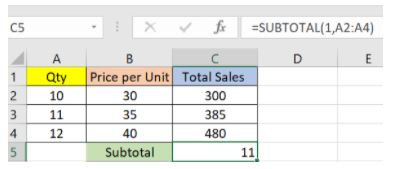
In the example above, we have performed the subtotal calculation on cells ranging from A2 to A4. As you can see, the function used is “=SUBTOTAL(1, A2: A4), in the subtotal list “1” refers to average. Hence, the above function will give the average of A2: A4 and the answer to it is 11, which is stored in C5.
Similarly, “=SUBTOTAL(4, A2: A4)” selects the cell with the maximum value from A2 to A4, which is 12. Incorporating “4” in the function provides the maximum result.
MODULUS
The MOD() function works on returning the remainder when a particular number is divided by a divisor. Let’s now have a look at the examples below for better understanding.
In the first example, we have divided 10 by 3. The remainder is calculated using the function “=MOD(A2,3)”. The result is stored in B2. We can also directly type “=MOD(10,3)” as it will give the same answer.
Similarly, here, we have divided 12 by 4. The remainder is 0 is, which is stored in B3.
6. POWER
The function “Power()” returns the result of a number raised to a certain power. Let’s have a look at the examples shown below:
As you can see above, to find the power of 10 stored in A2 raised to 3, we have to type “= POWER (A2,3)”. This is how power function works in Excel.
7. CEILING
Next, we have the ceiling function. The CEILING() function rounds a number up to its nearest multiple of significance.
The nearest highest multiple of 5 for 35.316 is 40.
8. FLOOR
Contrary to the Ceiling function, the floor function rounds a number down to the nearest multiple of significance.
the nearest lowest multiple of 5 for 35.316 is 35.
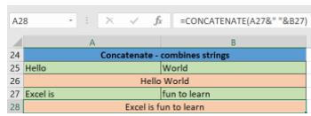
9. CONCATENATE
This function merges or joins several text strings into one text string. Given below are the different ways to perform this function.
In this example, we have operated with the syntax =CONCATENATE(A25, " ", B25)
In this example, we have operated with the syntax =CONCATENATE(A27&" "&B27)
Those were the two ways to implement the concatenation operation in Excel.
10. LEN
The function LEN() returns the total number of characters in a string. So, it will count the overall characters, including spaces and special characters. Given below is an example of the Len function
11. REPLACE
As the name suggests, the REPLACE() function works on replacing the part of a text string with a different text string.
The syntax is “=REPLACE(old_text, start_num, num_chars, new_text)”. Here, start_num refers to the index position you want to start replacing the characters with. Next, num_chars indicate the number of characters you want to replace.
Here, we are replacing A101 with B101 by typing “=REPLACE(A15,1,1,"B")”
Next, we are replacing A102 with A2102 by typing “=REPLACE(A16,1,1, "A2")”.
Finally, we are replacing Adam with Saam by typing “=REPLACE(A17,1,2, "Sa")”.
12. SUBSTITUTE
The SUBSTITUTE() function replaces the existing text with a new text in a text string.
The syntax is “=SUBSTITUTE(text, old_text, new_text, [instance_num])”.
Here, [instance_num] refers to the index position of the present texts more than once.
Here, we are substituting “I like” with “He likes” by typing “=SUBSTITUTE(A20, "I like","He likes")”.
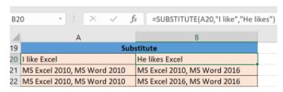
Next, we are substituting the second 2010 that occurs in the original text in cell A21 with 2016 by typing “=SUBSTITUTE(A21,2010, 2016,2)”.
Now, we are replacing both the 2010s in the original text with 2016 by typing “=SUBSTITUTE(A22,2010,2016)”.
13. LEFT, RIGHT, MID
The LEFT() function gives the number of characters from the start of a text string. Meanwhile, the MID() function returns the characters from the middle of a text string, given a starting position and length. Finally, the right() function returns the number of characters from the end of a text string.
In the example below, we use the function left to obtain the leftmost word on the sentence in cell A5.
Shown below is an example using the mid function.
Here, we have an example of the right function.
14. UPPER, LOWER, PROPER
The UPPER() function converts any text string to uppercase. In contrast, the LOWER() function converts any text string to lowercase. The PROPER() function converts any text string to proper case, i.e., the first letter in each word will be in uppercase, and all the other will be in lowercase.
Here, we have converted the text in A6 to a full uppercase one in A7.
Now, we have converted the text in A6 to a full lowercase one, as seen in A7.
Finally, we have converted the improper text in A6 to a clean and proper format in A7.
Exploring some date and time functions in Excel.
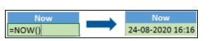
15. NOW()
The NOW() function in Excel gives the current system date and time.
The result of the NOW() function will change based on your system date and time.
16. TODAY()
The TODAY() function in Excel provides the current system date.
The function DAY() is used to return the day of the month. It will be a number between 1 to 31. 1 is the first day of the month, 31 is the last day of the month.
The MONTH() function returns the month, a number from 1 to 12, where 1 is January and 12 is December.
The YEAR() function, as the name suggests, returns the year from a date value.
17. TIME()
The TIME() function converts hours, minutes, seconds given as numbers to an Excel serial number, formatted with a time format.
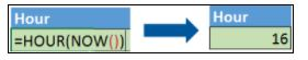
18. HOUR, MINUTE, SECOND
The HOUR() function generates the hour from a time value as a number from 0 to 23. Here, 0 means 12 AM and 23 is 11 PM.
The function MINUTE(), returns the minute from a time value as a number from 0 to 59
The SECOND() function returns the second from a time value as a number from 0 to 59.
9. DATEDIF
The DATEDIF() function provides the difference between two dates in terms of years, months, or days.
Below is an example of a DATEDIF function where we calculate the current age of a person based on two given dates, the date of birth and today’s date.
Now, let’s skin through a few critical advanced functions in Excel that are popularly used to analyze data and create reports.
20. VLOOKUP
Next up in this article is the VLOOKUP() function. This stands for the vertical lookup that is responsible for looking for a particular value in the leftmost column of a table. It then returns a value in the same row from a column you specify.
- Below are the arguments for the VLOOKUP function:
- lookup_value - This is the value that you have to look for in the first column of a table.
- table - This indicates the table from which the value is retrieved.
- col_index - The column in the table from the value is to be retrieved.
- range_lookup - [optional] TRUE = approximate match (default). FALSE = exact match.
We will use the below table to learn how the VLOOKUP function works.
If you wanted to find the department to which Stuart belongs, you could use the VLOOKUP function as shown below:
Here, A11 cell has the lookup value, A2: E7 is the table array, 3 is the column index number with information about departments, and 0 is the range lookup.
If you hit enter, it will return “Marketing”, indicating that Stuart is from the marketing department.
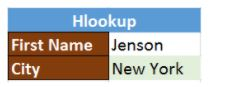
21. HLOOKUP
Similar to VLOOKUP, we have another function called HLOOKUP() or horizontal lookup. The function HLOOKUP looks for a value in the top row of a table or array of benefits. It gives the value in the same column from a row you specify.
Below are the arguments for the HLOOKUP function:
- lookup_value - This indicates the value to lookup.
- table - This is the table from which you have to retrieve data.
- row_index - This is the row number from which to retrieve data.
- range_lookup - [optional] This is a boolean to indicate an exact match or approximate match. The default value is TRUE, meaning an approximate match.
Given the below table, let’s see how you can find the city of Jenson using HLOOKUP.
Here, H23 has the lookup value, i.e., Jenson, G1:M5 is the table array, 4 is the row index number, 0 is for an approximate match.
Once you hit enter, it will return “New York”.
22. IF
The IF() function checks a given condition and returns a particular value if it is TRUE. It will return another value if the condition is FALSE.
In the below example, we want to check if the value in cell A2 is greater than 5. If it’s greater than 5, the function will return “Yes 4 is greater”, else it will return “No”.
In this case, it will return ‘No’ since 4 is not greater than 5.
‘IFERROR’ is another function that is popularly used. This function returns a value if an expression evaluates to an error, or else it will return the value of the expression.
Suppose you want to divide 10 by 0. This is an invalid expression, as you can’t divide a number by zero. It will result in an error.
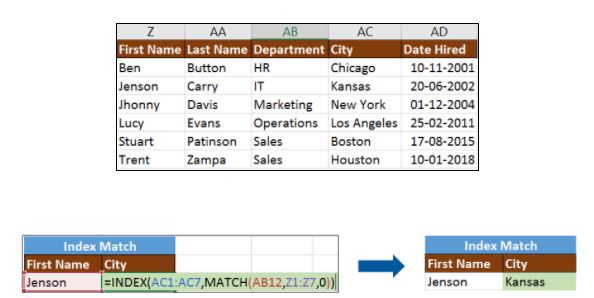
23. INDEX-MATCH
The INDEX-MATCH function is used to return a value in a column to the left. With VLOOKUP, you're stuck returning an appraisal from a column to the right. Another reason to use index-match instead of VLOOKUP is that VLOOKUP needs more processing power from Excel. This is because it needs to evaluate the entire table array which you've selected. With INDEX-MATCH, Excel only has to consider the lookup column and the return column.
Using the below table, let’s see how you can find the city where Jenson resides.
Now, let’s find the department of Zampa.

24. COUNTIF
The function COUNTIF() is used to count the total number of cells within a range that meet the given condition.
Below is a coronavirus sample dataset with information regarding the coronavirus cases and deaths in each country and region.
Let’s find the number of times Afghanistan is present in the table.
The COUNTIFS function counts the number of cells specified by a given set of conditions.
If you want to count the number of days in which the cases in India have been greater than 100. Here is how you can use the COUNTIFS function.
25. SUMIF
The SUMIF() function adds the cells specified by a given condition or criteria.
Below is the coronavirus dataset using which we will find the total number of cases in India till 3rd Jun 2020. (Our dataset has information from 31st Dec 2020 to 3rd Jun 2020).
The SUMIFS() function adds the cells specified by a given set of conditions or criteria.
Let’s find the total cases in France on those days when the deaths have been less than 100.